In this post I will introduce a much more efficient method for accounting block I/O latencies with eBPF on Linux. In my stress test, the “new biolatency” accounting method had 59x lower CPU and probe latency overhead compared to the current biolatency approach.
So I couldn’t help it and ended up putting 21 NVMe SSDs into one of my homelab servers. 8 of them are PCIe5 and the remaining 13 are PCIe4. The machine itself is a dual-socket AMD EPYC Genoa machine with 384 vCPUs and plenty of PCIe bandwidth (click to open SVG):

Without any low level tuning or even NUMA placement, fio was able to drive max 38.5M random read IOPS with smallest possible I/Os (512B and 4kB for some disks) and 173 GiB/s bandwidth with large 512kB random reads. In a single machine!
There’s enough PCIe and memory bandwidth to reach 35M IOPS even with 4kB block sizes used for all disks. With 8kB block size, you’d hit the PCIe/memory transfer bandwidth limit first (173 GiB/s in my setup). I’ll write about these things some other day, after running some serious database workloads on it.
I ran my tests on the latest Ubuntu 25.04 Server, with Linux 6.14 kernel. I used 18 fio worker threads per disk, total 18*21=378 threads. That’s pretty high concurrency, but my goal was to push this hardware to the max. Links to the scripts and settings I used are at the end of this post.
After verifying the aggregate IO throughput, the next steps were to drill down into IO latencies and see the latency distribution too (histograms). These days, the most widely used technique and tool for monitoring block IO latencies is biolatency from the iovisor/bcc toolset. Plenty of current observability tools and Prometheus exporters seem to use a similar pattern for gathering their latency histograms.
However, the moment I ran biolatency during my small IO stress test, the throughput dropped over 2x! The kernel mode CPU usage jumped much higher too as you see in the “biolatency OLD” section below:
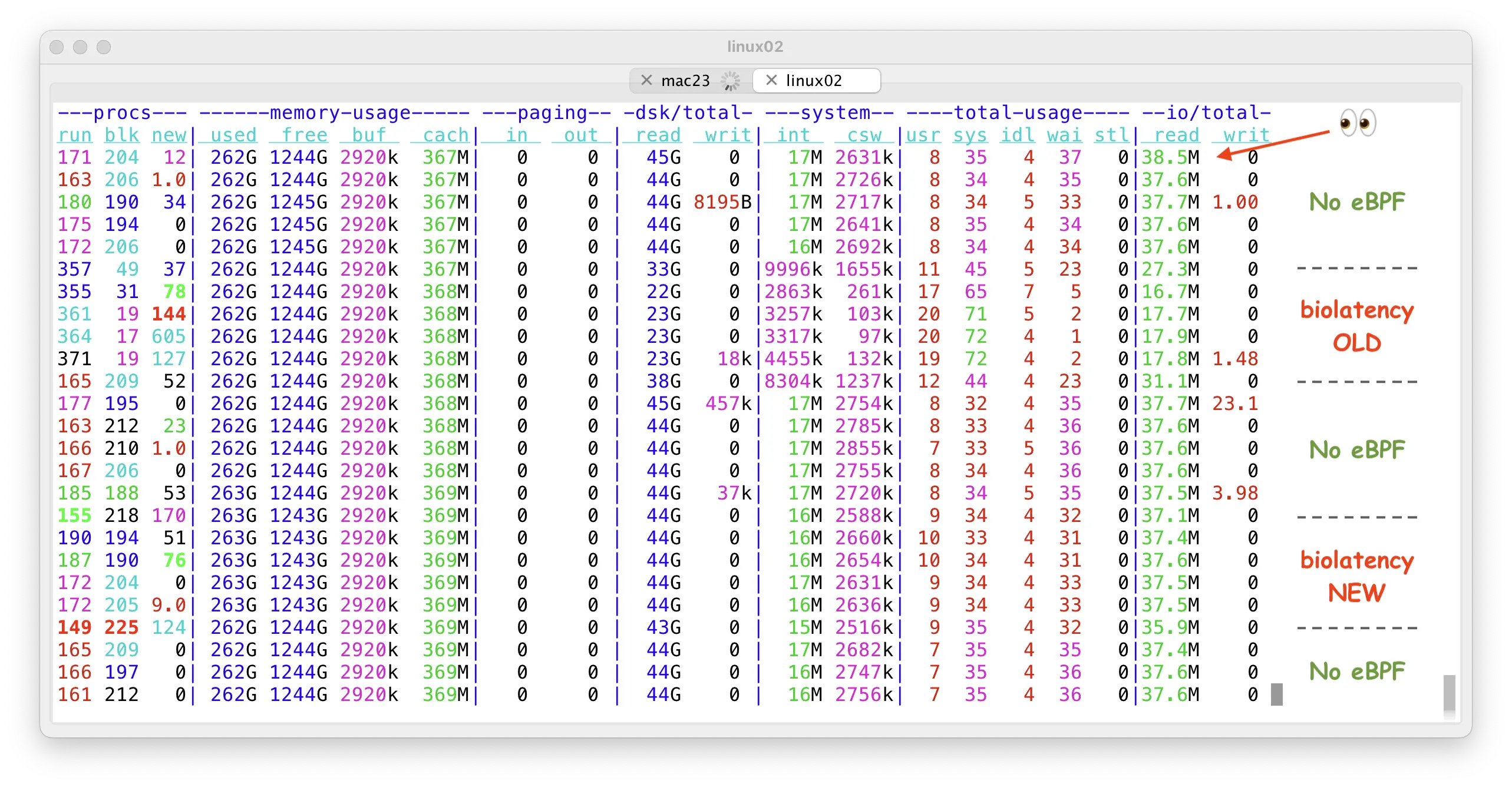
You might have noticed that there’s a section called “biolatency NEW” above too and its effect on throughput is barely noticeable! I will explain what I changed in a moment, first let’s see what is going on with the old approach.
I ran bpftop (by Netflix folks) that is a convenient frontend to the “bpftool prog profile” eBPF program profiling API (yes, since Linux 5.7, you can monitor your monitoring probes too).
Bpftop showed the following output:
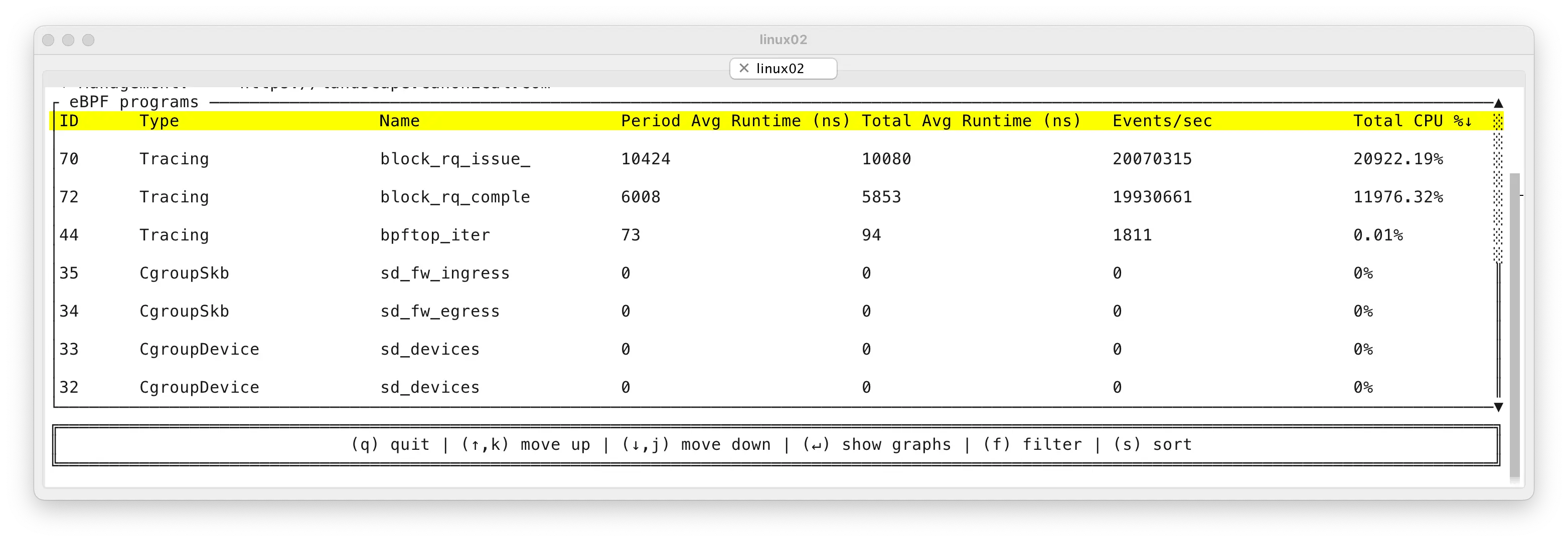
This shows me that the standard biolatency command uses at least two tracepoints: block_rq_issue and block_rq_complete. With -Q option, it can also use a block_rq_insert tracepoint, for tracking IO request insertions into the block device’s I/O queue at the OS level. But with locally attached NVMe disks and disks with plenty of hardware IO dispatch capacity this stage is bypassed, so this tracepoint is not hit and won’t make its way to the top of the on-screen output.
So what’s going on here? When you look into the Events/sec column, we are hitting the IO issue & completion tracepoints about 20M times per second. Forgive the inconsistency between this ~20M and the ~17.8M IO rate shown before - I took many screenshots over many tests, there may be a minor mixup across my test variations.
If you look into the Avg Runtime (ns) columns above, you see that each IO incurred an eBPF probe cost twice. First about 10 microseconds when tracking the IO issuing phase and then about 6 microseconds for IO completion. That’s about 16 microseconds of CPU (and latency) overhead per IO! This is actually quite significant overhead when you do millions of IOPS per server. Also, small IO latency on modern NVMe SSDs is measured in tens of microseconds these days, so adding 16 microseconds (or even only 6 microseconds) of latency just for monitoring dashboards does not feel that good.
Finally, the Total CPU % column in the top right shows 20922% + 11976% of CPU time used for these eBPF tracepoints only. This percentage metric shows total CPU time used across all CPUs in the system, normalized to a single CPU’s time. So we can infer that 20922% of a CPU time means that we used ~209 CPUs (out of 384) just for handling the top tracepoint! And ~119 CPUs for the second one.
Of course my test is a pretty crazy synthetic stress test of doing only IOs without useful processing of the data, but this is what you get when you scale the eBPF program concurrency to the extreme, without scaling the control flow and underlying data structures to match the increased needs, especially on NUMA systems with lots of CPUs.
So what’s the bottleneck?
There are 3 noteworthy items in the (current) biolatency.bpf.c code:
1. I/O start time recording map
The old approach uses a globally visible hashmap “start”, organized by IO request address (struct request *) to keep track of I/O start times for computing a delta later:
struct {
  __uint(type, BPF_MAP_TYPE_HASH);
  __uint(max_entries, MAX_ENTRIES);
  __type(key, struct request *);
  __type(value, u64);
} start SEC(".maps");
The IO insert/issue tracepoints have to insert their current timestamp into this hashtable every time a new IO is issued:
bpf_map_update_elem(&start, &rq, &ts, 0);
Once the IO completes, the IO completion handler takes the completing IO request address from its tracepoint argument, looks up the start time and calculates delta between the start time and its current time. This is roughly the I/O latency - that inevitably includes some CPU processing overhead:
  tsp = bpf_map_lookup_elem(&start, &rq);
  if (!tsp)
    return 0;

  delta = (s64)(ts - *tsp);
This “start” map has to be a globally visible structure, it can not be a per-CPU map as the IO request may be completed on a different CPU from wherever it was submitted from. The IO is typically completed on the CPU where the hardware interrupt handler happens to run.
2. Aggregated latency bucket counter map
Now that we know the individual IO’s latency (delta), the IO completion handler also has to increment the respective latency bucket in the “hists” map:
struct {
  __uint(type, BPF_MAP_TYPE_HASH);
  __uint(max_entries, MAX_ENTRIES);
  __type(key, struct hist_key);
  __type(value, struct hist);
} hists SEC(".maps");
This involves multiple hashmap lookups and updates as you see:
  histp = bpf_map_lookup_elem(&hists, &hkey);
  if (!histp) {
    bpf_map_update_elem(&hists, &hkey, &initial_hist, 0);
    histp = bpf_map_lookup_elem(&hists, &hkey);
    if (!histp)
      goto cleanup;
  }
… that is finally followed by a synchronous (atomic) increment operation where the CPU & cache coherency layer guarantee that no increments get lost. Even though no spinlocks are used, this can be especially expensive on NUMA machines with multiple CPU sockets and even modern single-socket machines with multiple independent core complexes (like my AMD EPYC) will feel the effect too.
__sync_fetch_and_add(&histp->slots[slot], 1);
And finally, once the IO completion is handled, we’ll need to remove this IO request from the “start” map. This memory address will likely be quickly reused by an upcoming new IO request and the whole process will repeat.
bpf_map_delete_elem(&start, &rq);
That’s a lot of inserts, lookups and deletions of objects from a hash map. An eBPF hash map is not a simple structure and certainly when you have up to 384 programs concurrently accessing & modifying this table, there will be traffic!
3. Hash table size
The old biolatency tool has this hashmap size by default:
#define MAX_ENTRIES 10240
Just to be fair, I did increase it from 10240 to 262144 when I was testing the old biolatency code to account for increased concurrency due to the number of CPUs and number of concurrent in-flight IOs due to the number of disks in the system.
But funnily, since in the new biolatency we removed that “start” map completely and the “hists” map itself would contain just a few dozen values per disk/IO request flag (if breakdown by disk/iorq flag was enabled), I did actually shrink the hashmap size to 512 in my later tests.
How did I fix it?
I will start by showing you the bpftop output from after fixing the bottlenecks, running the same stress test:
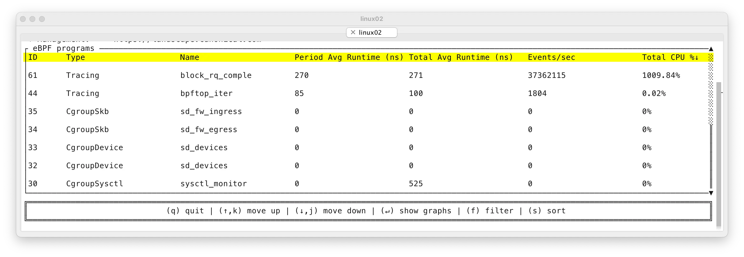
Now we have only one tracepoint activated per IO instead of two. And each activation of the IO completion tracepoint takes only 271 nanoseconds on average, instead of microseconds. Therefore we are using “only” ~10 CPUs for accounting all 37M IOs per second. That’s 59x more efficient compared to the previous approach (at least for my crazy stress test :-).
Because of my earlier work, I was aware that Linux block layer’s struct request actually keeps track of I/O insertion and issue timestamps in nanoseconds, for every I/O request (since kernel 2.6.35).
  /* Time that this request was allocated for this IO. */
  u64 start_time_ns;
  /* Time that I/O was submitted to the device. */
  u64 io_start_time_ns;
As Linux itself keeps track of the IO insert & issue times, we don’t need to maintain our own, shared “start” hashmap at all. No need for ultrafrequent hashtable insertions, lookups and deletes. In fact, the whole block_rq_issue tracepoint is not needed at all!
So I just removed the insert, issue tracepoints and the “start” hashmap as the first step. I would just access the IO request structure in the IO completion tracepoint and read the device number, IO request flags and the IO start timestamps in one go. That solved the issue #1.
Now that we are in the IO completion tracepoint and have calculated the delta between IO start and completion (current time), we still need to increment a counter in the respective latency bucket in the final output map.
Unlike the previous “start” map, the latency bucket map does not need to be visible to the entire system, just local CPU wherever the tracepoint runs is OK. We’d just roll up the aggregates in all individual CPU-level buckets to the final system-wide histogram. In other words, I used BPF_MAP_TYPE_PERCPU_HASH for the “hists” map, without needing any structural changes in the eBPF code (the userspace code has to read and clear all 384 per-CPU maps now, instead of just a single global one). That solved the issue #2. And the issue #3 became a non-issue, as the remaining output histogram map was CPU-local now and since it’s an aggregated summary, it doesn’t contain that many items anyway.
All this gives us the following result:
tanel@linux02:~/dev/bcc/libbpf-tools$ sudo ./biolatency 10 1
Tracing block device I/O... Hit Ctrl-C to end.

DEBUG: ncpus=384, sizeof(struct hist)=216, attempting to allocate 82944 bytes for per-CPU data
DEBUG: Checking map fd 4 for keys...
DEBUG: Starting map processing loop.
DEBUG: Processing key: dev=0 flags=0
DEBUG: Aggregated total count for this key: 373422791
     usecs               : count    distribution
         0 -> 1          : 0        |                                        |
         2 -> 3          : 0        |                                        |
         4 -> 7          : 0        |                                        |
         8 -> 15         : 136      |                                        |
        16 -> 31         : 16209    |                                        |
        32 -> 63         : 776709   |                                        |
        64 -> 127        : 7216424  |**                                      |
       128 -> 255        : 18213454 |*******                                 |
       256 -> 511        : 16881973 |******                                  |
       512 -> 1023       : 42142038 |****************                        |
      1024 -> 2047       : 90072892 |***********************************     |
      2048 -> 4095       : 100878032 |****************************************|
      4096 -> 8191       : 52073668 |********************                    |
      8192 -> 16383      : 28106291 |***********                             |
     16384 -> 32767      : 12500205 |****                                    |
     32768 -> 65535      : 4539084  |*                                       |
     65536 -> 131071     : 5676     |                                        |
DEBUG: End of map iteration (get_next_key -> ENOENT).
DEBUG: Starting map cleanup loop.
DEBUG: Finished map cleanup loop.
Exiting.
The dstat output you already saw earlier in this post:
The fastest way to do something is to not do it at all!
Code
Important: This code is beta do not use in production yet!. It’s because of two glitches that I saw with the new approach. One was about showing an occasional IO outlier that the DM module causes (and the old biolatency dropped/ignored) and the other one occasionally caused a multi-second livelock-like “hiccup” when cleaning up all 384 per-CPU “hists” maps while the heavy IO load was still going on. I think the issue is not in my modifications, but rather about a glitch/bug in Linux eBPF subsystem behavior with lots of CPUs. I will research this more and blog about it & raise a bug, before declaring this approach production ready.
You can see the updated files here:
You can just copy them to the iovisor/bcc/libbpf-tools/ directory (back up the previous ones) and build there.
I also plan to raise a PR to the original iovisor/BCC repo, once its ready.
Note that my recently announced xCapture v3 & DuckDB-based Linux performance analysis tool still uses the “old approach”, thus is not as efficient as it could be. The challenge is in being able to see the IO originator PID (or task pointer) in addition to the IO start times. Linux currently (unfortunately) does not save the IO originator info into its “struct request”, so a more creative approach is needed. Stay tuned!

Further reading
If you want to read more case studies about how I pushed the limits of hardware and software, check out these two posts: